Bias Estimation

On the Teledyne/e2v CCD230-42 sensors used by the MSFC camera, there are 50 blank columns at the start of each row, and 2 overscan columns at the end of each row. This report will investigate which combination of blank and overscan columns results in the best estimation of the bias using a single dark frame from the EUV Snapshot Imaging Spectrograph (ESIS) 2019 flight.

import IPython.display
import numpy as np
import astropy.units as u
import astropy.visualization
import matplotlib.pyplot as plt
import named_arrays as na
import msfc_ccd

astropy.visualization.quantity_support();

Load a single dark from the ESIS 2019 flight.

dark = msfc_ccd.fits.open(msfc_ccd.samples.path_dark_esis1)

fig, ax = plt.subplots(
    figsize=(8, 4),
    constrained_layout=True,
)
im = na.plt.imshow(
    dark.outputs.value,
    axis_x=dark.axis_x,
    axis_y=dark.axis_y,
    ax=ax,
)
ax.set_xlabel("detector $x$ (pix)")
ax.set_ylabel("detector $y$ (pix)")
plt.colorbar(im.ndarray.item(), ax=ax, label="signal (DN)");

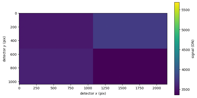
Split the dark image up into separate images for each tap.

taps = dark.taps

Save the names of the logical axes corresponding to changing tap index

axis_tap_x = taps.axis_tap_x
axis_tap_y = taps.axis_tap_y

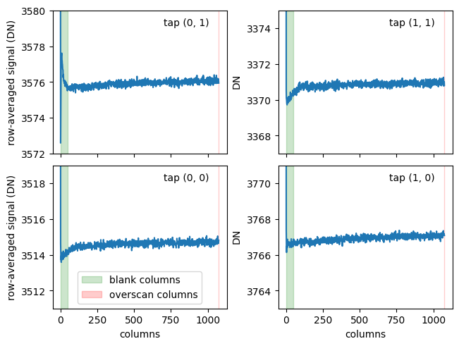
Plot the average dark signal for each column in each tap, along with the blank and overscan regions for each tap. Notice that the signal in the blank columns is often a poor representation of the average signal along all the columns.

fig, ax = na.plt.subplots(
    axis_rows=axis_tap_y,
    axis_cols=axis_tap_x,
    nrows=taps.shape[axis_tap_y],
    ncols=taps.shape[axis_tap_x],
    sharex=True,
    constrained_layout=True,
)
na.plt.plot(
    taps.outputs.mean_trimmed(.01, taps.axis_y),
    axis=taps.axis_x,
    ax=ax,
)
na.plt.set_ylim(
    bottom=taps.outputs.percentile(5, axis=taps.axis_xy),
    top=taps.outputs.percentile(95, axis=taps.axis_xy),
    ax=ax,
)
na.plt.axvspan(
    xmin=0,
    xmax=taps.camera.sensor.num_blank,
    color="green",
    alpha=0.2,
    ax=ax,
    label="blank columns",
)
na.plt.axvspan(
    xmin=taps.num_x - taps.camera.sensor.num_overscan,
    xmax=taps.num_x,
    color="red",
    alpha=0.2,
    ax=ax,
    label="overscan columns",
)
na.plt.set_ylabel("row-averaged signal (DN)", ax[{axis_tap_x: 0}])
na.plt.set_xlabel("columns", ax=ax[{axis_tap_y: 0}])
na.plt.text(
    x=0.9,
    y=0.95,
    s=taps.label,
    ax=ax,
    transform=na.plt.transAxes(ax),
    ha="right",
    va="top",
)
ax.ndarray.flat[0].legend();

With this in mind, we’ll use msfc_ccd.TapData.bias() to estimate the bias from only the blank columns or the overscan columns.

bias_blank = taps.bias(num_blank=None, num_overscan=0)
bias_overscan = taps.bias(num_blank=0, num_overscan=None)

Then, we’ll subtract the bias estimated using these two regions from each tap image,

unbiased_blank = taps - bias_blank
unbiased_overscan = taps - bias_overscan

and smooth the result slightly to make it easier to visualize.

kwargs_filter = dict(
    size={taps.axis_x: 11, taps.axis_y: 11},
    proportion=0.05,
)
unbiased_blank = na.ndfilters.trimmed_mean_filter(unbiased_blank, **kwargs_filter)
unbiased_overscan = na.ndfilters.trimmed_mean_filter(unbiased_overscan, **kwargs_filter)

Finally, we’ll take the tap images and reconstruct them into a bias-subtracted dark frame.

dark_blank = dark.from_taps(unbiased_blank)
dark_overscan = dark.from_taps(unbiased_overscan)

Now, if we make a histogram of the smoothed, bias-subtracted tap image pixel values,

kwargs_hist = dict(
    axis=taps.axis_xy,
    bins=na.arange(-2, 2, "xy", .1) * u.DN,
    density=True,
)
hist_blank = na.histogram(unbiased_blank.outputs, **kwargs_hist)
hist_overscan = na.histogram(unbiased_overscan.outputs, **kwargs_hist)

fig, ax = na.plt.subplots(
    axis_rows=axis_tap_y,
    axis_cols=axis_tap_x,
    nrows=taps.shape[axis_tap_y],
    ncols=taps.shape[axis_tap_x],
    sharex=True,
    sharey=True,
    constrained_layout=True,
)
na.plt.stairs(
    hist_blank.inputs,
    hist_blank.outputs,
    ax=ax,
    axis="xy",
    label="blank",
)
na.plt.stairs(
    hist_overscan.inputs,
    hist_overscan.outputs,
    ax=ax,
    axis="xy",
    label="overscan",
)
na.plt.text(
    x=0.95,
    y=0.95,
    s=taps.label,
    ax=ax,
    transform=na.plt.transAxes(ax),
    ha="right",
    va="top",
)
na.plt.axvline(0, ax=ax, color="black", linestyle="--")
na.plt.set_ylabel("probability density", ax[{axis_tap_x: 0}])
na.plt.set_xlabel("smoothed signal (DN)", ax=ax[{axis_tap_y: 0}])
ax[{axis_tap_x: 0, axis_tap_y: ~0}].ndarray.legend(loc="upper left");

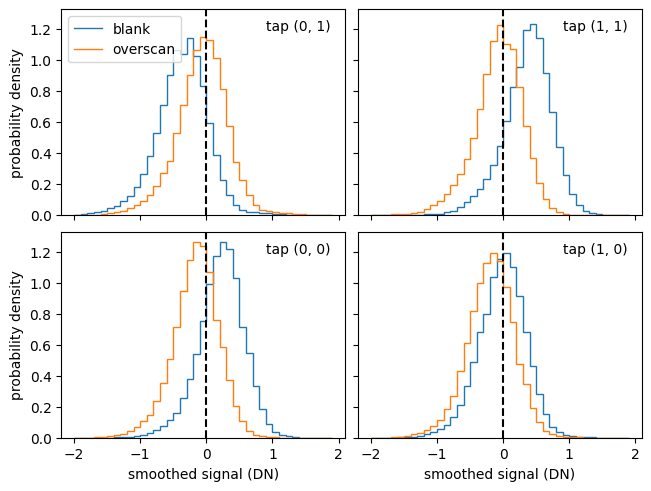
we can see that the bias based on the overscan pixels does a much better job of centering the distribution around zero. In fact, if we compare the trimmed mean of the blank-bias-subtracted taps

unbiased_blank.outputs.mean_trimmed(0.01, taps.axis_xy)

ScalarArray(
    ndarray=[[ 0.22037477, -0.02296992],
             [-0.36443315,  0.36416235]] DN,
    axes=('tap_y', 'tap_x'),
)

to the trimmed mean of the overscan-bias-subtracted taps,

unbiased_overscan.outputs.mean_trimmed(0.01, taps.axis_xy)

ScalarArray(
    ndarray=[[-0.16158677, -0.19223915],
             [-0.06916392, -0.07476073]] DN,
    axes=('tap_y', 'tap_x'),
)

we can see that the average is much closer to zero using the bias computed from the overscan pixels.

One final visualization we can do is blink the blank-bias-subtracted dark image against the overscan-bias-subtracted dark image to compare.

fig, ax = plt.subplots(constrained_layout=True)
colorizer = plt.Colorizer(
    norm=plt.Normalize(
        vmin=-1,
        vmax=1,
    ),
)
ani = na.plt.pcolormovie(
    na.ScalarArray(
        ndarray=np.array(["blank", "overscan"]),
        axes="blink",
    ),
    dark.inputs.pixel.x,
    dark.inputs.pixel.y,
    C=na.stack(
        arrays=[dark_blank.outputs, dark_overscan.outputs],
        axis="blink",
    ),
    axis_time="blink",
    ax=ax,
    kwargs_pcolormesh=dict(
        colorizer=colorizer,
    ),
    kwargs_animation=dict(
        interval=1000,
    )
)

ax.set_xlabel("detector $x$ (pix)")
ax.set_ylabel("detector $y$ (pix)")
plt.colorbar(
    mappable=plt.cm.ScalarMappable(colorizer=colorizer),
    ax=ax,
    label="signal (DN)"
)
plt.close(fig)
IPython.display.HTML(ani.to_jshtml())

Once Loop Reflect

This shows that the overscan-bias-subtracted dark image is much better at removing the seams in between each tap.

In conclusion, we recommend to only use the overscan columns to compute the bias, unless other MSFC cameras than the single one studied here have much different behavior. For that reason, we have set the arguments of msfc_ccd.TapData.bias() to use only the overscan columns by default.