Bias Estimation

On the Teledyne/e2v CCD230-42 sensors used by the MSFC camera, there are 50 blank columns at the start of each row, and 2 overscan columns at the end of each row. msfc_ccd.TapData.bias() estimates the bias of each tap using the 25 blank columns closest to the active pixels.

The blank columns are read out before any of the active pixels in each row, so they do not depend on the brightness of the image, and using 25 of them makes the noise in the bias about 0.04 DN per image. The first 25 blank columns are ignored since they contain a transient from the start of each row, and the overscan columns are ignored since they contain charge deferred from the active pixels.

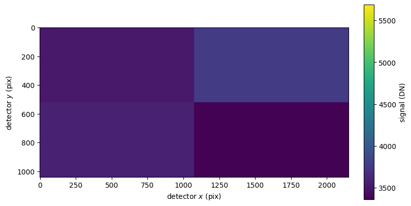
This report demonstrates each of these points using an image of a diffuse LED source and a dark image captured two minutes later, both gathered by the ESIS channel 1 camera during the linearity test on 2017-07-12.

import astropy.visualization
import matplotlib.pyplot as plt
import named_arrays as na
import msfc_ccd

astropy.visualization.quantity_support();

Load the LED image and the dark image.

led = msfc_ccd.fits.open(msfc_ccd.samples.path_led_esis1)
dark = msfc_ccd.fits.open(msfc_ccd.samples.path_led_dark_esis1)

fig, ax = plt.subplots(
    figsize=(8, 4),
    constrained_layout=True,
)
im = na.plt.imshow(
    led.outputs.value,
    axis_x=led.axis_x,
    axis_y=led.axis_y,
    ax=ax,
)
ax.set_xlabel("detector $x$ (pix)")
ax.set_ylabel("detector $y$ (pix)")
plt.colorbar(im.ndarray.item(), ax=ax, label="signal (DN)");

Split both images up into separate images for each tap, and save the names of the logical axes.

taps = led.taps
taps_dark = dark.taps

axis_x = taps.axis_x
axis_y = taps.axis_y
axis_tap_x = taps.axis_tap_x
axis_tap_y = taps.axis_tap_y

num_x = taps.num_x
num_blank = taps.camera.sensor.num_blank
num_overscan = taps.camera.sensor.num_overscan

The blank columns

Plot the average signal in each of the blank columns of the dark image, relative to the bias.

fig, ax = na.plt.subplots(
    axis_rows=axis_tap_y,
    axis_cols=axis_tap_x,
    nrows=taps.shape[axis_tap_y],
    ncols=taps.shape[axis_tap_x],
    sharex=True,
    sharey=True,
    constrained_layout=True,
)
na.plt.stairs(
    na.arange(0, num_blank + 1, axis=axis_x) - 0.5,
    taps_dark.unbiased.outputs[{axis_x: slice(0, num_blank)}].mean(axis_y),
    axis=axis_x,
    ax=ax,
    baseline=None,
)
na.plt.axvspan(
    xmin=num_blank - 25 - 0.5,
    xmax=num_blank - 0.5,
    color="green",
    alpha=0.2,
    ax=ax,
    label="columns used for the bias",
)
na.plt.set_ylim(-5, 5, ax=ax)
na.plt.set_ylabel("row-averaged signal (DN)", ax[{axis_tap_x: 0}])
na.plt.set_xlabel("columns", ax=ax[{axis_tap_y: 0}])
na.plt.text(
    x=0.95,
    y=0.95,
    s=taps.label,
    ax=ax,
    transform=na.plt.transAxes(ax),
    ha="right",
    va="top",
)
ax.ndarray.flat[0].legend(loc="lower right");

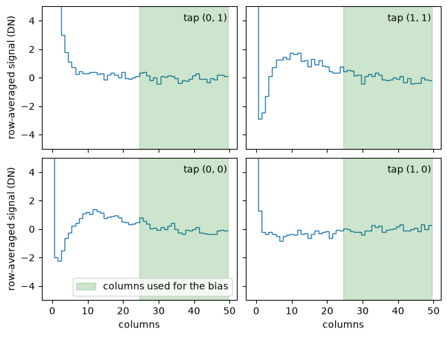
Every row starts with a transient which is tens of DN in the first column and takes about 25 columns to settle, which is why only the 25 blank columns closest to the active pixels are used.

To check that these columns do not depend on the brightness of the image, subtract the dark image from the LED image,

signal = taps.unbiased.outputs - taps_dark.unbiased.outputs

and plot the average of the result in each of the blank columns, along with the first few active columns for comparison.

fig, ax = na.plt.subplots(
    axis_rows=axis_tap_y,
    axis_cols=axis_tap_x,
    nrows=taps.shape[axis_tap_y],
    ncols=taps.shape[axis_tap_x],
    sharex=True,
    sharey=True,
    constrained_layout=True,
)
num = 5
na.plt.stairs(
    na.arange(0, num_blank + num + 1, axis=axis_x) - 0.5,
    signal[{axis_x: slice(0, num_blank + num)}].mean(axis_y),
    axis=axis_x,
    ax=ax,
    baseline=None,
)
na.plt.axvspan(
    xmin=num_blank - 25 - 0.5,
    xmax=num_blank - 0.5,
    color="green",
    alpha=0.2,
    ax=ax,
    label="columns used for the bias",
)
na.plt.set_yscale("symlog", ax=ax, linthresh=1)
na.plt.set_ylabel("row-averaged signal (DN)", ax[{axis_tap_x: 0}])
na.plt.set_xlabel("columns", ax=ax[{axis_tap_y: 0}])
na.plt.text(
    x=0.05,
    y=0.95,
    s=taps.label,
    ax=ax,
    transform=na.plt.transAxes(ax),
    ha="left",
    va="top",
)
ax.ndarray.flat[0].legend(loc="center left");

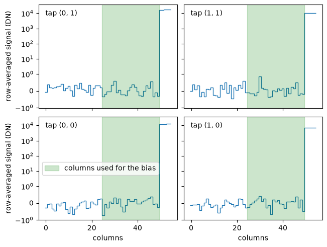
The blank columns stay within the noise of zero, right up to the first active column, which contains more than 10,000 DN. The transient at the start of each row is also unchanged by the LED, since it has been removed by subtracting the dark image.

The overscan columns

The overscan columns are read out after the active pixels in each row. If we plot the same difference between the LED image and the dark image for the last few columns of each tap,

fig, ax = na.plt.subplots(
    axis_rows=axis_tap_y,
    axis_cols=axis_tap_x,
    nrows=taps.shape[axis_tap_y],
    ncols=taps.shape[axis_tap_x],
    sharex=True,
    sharey=True,
    constrained_layout=True,
)
num = 4
na.plt.stairs(
    na.arange(num_x - num_overscan - num, num_x + 1, axis=axis_x) - 0.5,
    signal[{axis_x: slice(-num_overscan - num, None)}].mean(axis_y),
    axis=axis_x,
    ax=ax,
    baseline=None,
)
na.plt.axvspan(
    xmin=num_x - num_overscan - 0.5,
    xmax=num_x - 0.5,
    color="red",
    alpha=0.2,
    ax=ax,
    label="overscan columns",
)
na.plt.set_yscale("log", ax=ax)
na.plt.set_ylabel("row-averaged signal (DN)", ax[{axis_tap_x: 0}])
na.plt.set_xlabel("columns", ax=ax[{axis_tap_y: 0}])
na.plt.text(
    x=0.05,
    y=0.05,
    s=taps.label,
    ax=ax,
    transform=na.plt.transAxes(ax),
    ha="left",
    va="bottom",
)
ax.ndarray.flat[0].legend();

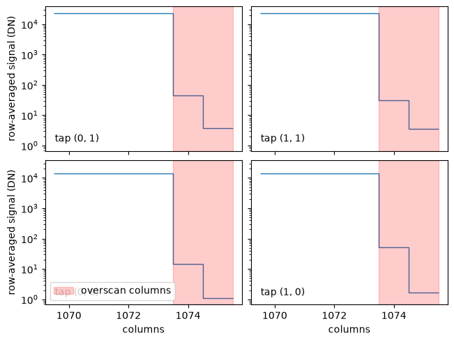
we can see that the first overscan column contains tens of DN, and the second overscan column contains a few DN. This is charge deferred from the last active pixels in each row by the imperfect charge transfer efficiency of the serial register. The ratio of the first overscan column to the last active column is

edge = signal[{axis_x: ~num_overscan}]
overscan_1 = signal[{axis_x: ~1}]
overscan_2 = signal[{axis_x: ~0}]

ratio_1 = overscan_1.mean(axis_y) / edge.mean(axis_y)
ratio_1

ScalarArray(
    ndarray=[[0.00103915, 0.00367508],
             [0.00190626, 0.00131425]] ,
    axes=('tap_y', 'tap_x'),
)

and the ratio of the second overscan column to the last active column is about ten times smaller.

ratio_2 = overscan_2.mean(axis_y) / edge.mean(axis_y)
ratio_2

ScalarArray(
    ndarray=[[7.69486430e-05, 1.14486647e-04],
             [1.60287903e-04, 1.51470678e-04]] ,
    axes=('tap_y', 'tap_x'),
)

Since the LED does not illuminate the sensor evenly, the last active column changes along each tap, and the first overscan column follows it closely.

kwargs_filter = dict(
    size={axis_y: 51},
    proportion=0.05,
)
rows = na.arange(0, taps.num_y, axis=axis_y)

fig, ax = na.plt.subplots(
    axis_rows=axis_tap_y,
    axis_cols=axis_tap_x,
    nrows=taps.shape[axis_tap_y],
    ncols=taps.shape[axis_tap_x],
    sharex=True,
    constrained_layout=True,
)
na.plt.plot(
    rows,
    na.ndfilters.trimmed_mean_filter(overscan_1, **kwargs_filter),
    axis=axis_y,
    ax=ax,
    label="first overscan column",
)
na.plt.plot(
    rows,
    na.ndfilters.trimmed_mean_filter(overscan_2, **kwargs_filter),
    axis=axis_y,
    ax=ax,
    label="second overscan column",
)
na.plt.plot(
    rows,
    ratio_1 * na.ndfilters.trimmed_mean_filter(edge, **kwargs_filter),
    axis=axis_y,
    ax=ax,
    color="black",
    linestyle="--",
    label="scaled last active column",
)
na.plt.set_ylabel("smoothed signal (DN)", ax[{axis_tap_x: 0}])
na.plt.set_xlabel("rows", ax=ax[{axis_tap_y: 0}])
na.plt.text(
    x=0.95,
    y=0.5,
    s=taps.label,
    ax=ax,
    transform=na.plt.transAxes(ax),
    ha="right",
    va="center",
)
handles, labels = ax.ndarray.flat[0].get_legend_handles_labels()
fig.legend(handles, labels, loc="outside upper center", ncols=3);

A bias computed from the overscan columns would therefore depend on the brightness of the image. Between the dark image and the LED image it changes by

kwargs_overscan = dict(num_blank=0, num_overscan=None)
taps.bias(**kwargs_overscan).outputs - taps_dark.bias(**kwargs_overscan).outputs

ScalarArray(
    ndarray=[[ 8.39230769, 27.44423077],
             [24.60769231, 18.04423077]] DN,
    axes=('tap_y', 'tap_x'),
)

while the bias computed from the blank columns changes by

taps.bias().outputs - taps_dark.bias().outputs

ScalarArray(
    ndarray=[[0.48461538, 0.45584615],
             [0.62823077, 1.01976923]] DN,
    axes=('tap_y', 'tap_x'),
)

which includes any genuine drift of the bias during the two minutes between the images.

Dark subtraction

The blank columns are offset from the dark level of the active pixels. For the dark image, the average of the bias-subtracted active pixels in each tap is

taps_dark.unbiased.active.outputs.mean_trimmed(0.01, axis=taps.axis_xy)

ScalarArray(
    ndarray=[[-0.30180011,  0.24092492],
             [ 0.12597406, -0.29058253]] DN,
    axes=('tap_y', 'tap_x'),
)

This offset is different for each tap, so it would leave faint seams between the taps, but it does not change from one image to the next. It is removed, along with the dark current, by subtracting a dark image which has had its bias removed in the same way.